![]()
![]()
![]()
![]()
Methods for analyzing interactions within a system include flow diagrams, matrices, and models.
· Flow diagrams
Figure 5 is one of the simpler diagrams and illustrates cause/effect relationships. Although useful as a first approximation, it does not explicitly consider the processes involved, and it defines a particular action in only one way. The consequences of a variation in the design of a dam or some other action can be taken into account only by constructing another, different cause/effect diagram. In other words, the diagram permits only one output option, a decrease in fish production, to be considered.
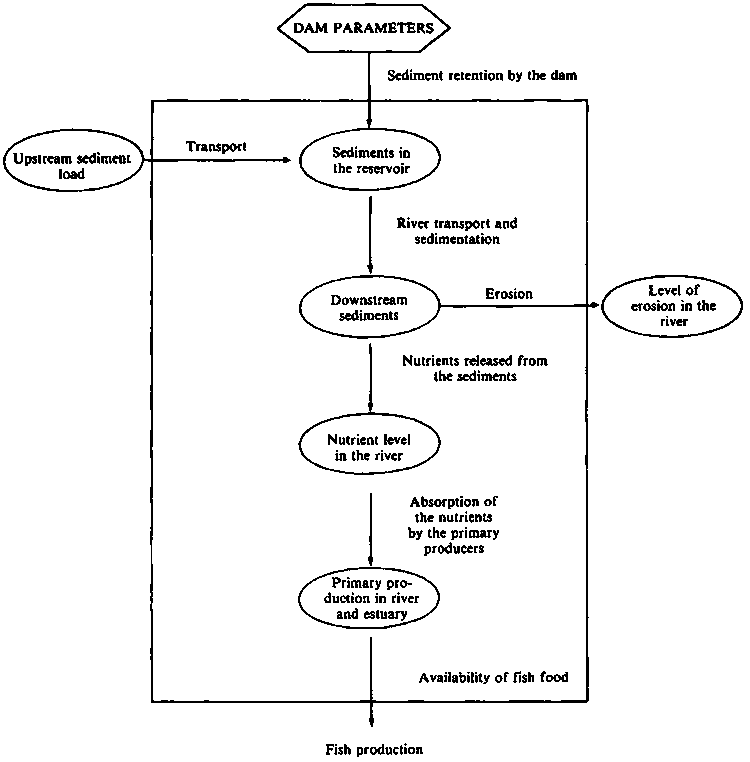
Figure 11 is a flow diagram based on the same situation as that in Figure 5. Each block indicates a process, the arrows indicate input or output variables, and the hexagon indicates an intervention. Note that the large box contains several more elementary boxes, each with its own inputs and outputs. In order to predict the effect of the dam on an output variable, such as the production of fish or a change in the state of stream erosion, it is necessary to consider a group of intermediate variables and processes. Thus Figure 11 is more general than Figure 5 because it permits representation of alternative effects in the same diagram. For example, modification in the dam structure or additions of nutrients to the river through the return of irrigation water may finally result in an increase rather than a decrease in fish production.
An alternative way to represent the same system is given in Figure 12. However, the arrows now represent processes or transformations and the ovals represent the variables. Note that this is the opposite representation of the flow diagram in Figure 11.
Finally, Figure 13 shows a simplified version of the same situation but the relationships are "monotonous." That is, the effect of one variable on another is always in the same direction. Thus the plus sign (+) between the variables "Nutrient level in the river" and "Primary production in river and estuary" indicates that, if the addition of nutrients is increased, the primary production is also increased and, if the addition is decreased, the primary production is likewise decreased. The minus sign (-) at the variable "Downstream sediment load" and "Level of river erosion" implies that, if the sediments increase, the erosion decreases and vice versa. Use of this type of diagram allows representation of the transfer of the negative or positive effects of the input variables to the output variables.
Figure 11. Flow diagram showing the effects of a dam on fish production and stream erosion

Figure 12. Flow diagram showing the effects of a dam on fish production and stream erosion
The disadvantage of this type of focus is that the relationship may not be "monotonous." At times the effect of one variable on another may change depending on the size of the variable. For example, an increase in primary production can increase the fish production but, at certain levels, an "excess" of primary production intensifies the process of eutrofication which may, in turn, provoke a decrease in fish production.
· Matrices
An alternative way of representing flow diagrams is with a matrix. For example, the matrix in Figure 14 represents the diagram in Figure 11 and indicates with a number one (1) the existence of interactions between horizontal and vertical coordinates, but says nothing of the types of interactions. The matrix in Figure 15 is similar to that of Figure 14 but, in addition, it indicates the types of processes by which the horizontal variable transforms the vertical variable. For example, PP (Primary Production) influences FP (Fish Production) through f (availability of fish food). Figure 16 is a matrix representing the flow diagram in Figure 13 where the signs in the matrix cells indicate the directions of interactions between variables.
The mechanism for transferring inputs to outputs for each individual block can vary depending on the subject, the availability of information, and the required precision. As a simple hypothetical example consider the last block in Figure 11 which represents the supply of food for the fish population, a process connecting primary production with fish population. The transformation could be defined in several ways at different orders of complexity and precision.
a) A simple qualitative description where the required inputs are an increase or decrease in primary production and the outputs generated are an increase or decrease in fish production is presented in Figure 17.
- The fish population increases to an undetermined degree if primary production increases; and- The fish population decreases to an undetermined degree if primary production decreases.
Figure 13. Flow diagram showing the effects of a dam on fish production where the effects are monotonous

Figure 14. Matrix representing the relationships in Figure 11
|
|
DP |
US |
RS |
DS |
RE |
NL |
PP |
FP |
|
DP |
|
|
I |
|
|
|
|
|
|
US |
|
|
I |
|
|
|
|
|
|
RS |
|
|
|
I |
|
|
|
|
|
DS |
|
|
|
|
I |
I |
|
|
|
RE |
|
|
|
|
|
|
|
|
|
NL |
|
|
|
|
|
|
I |
|
|
PP |
|
|
|
|
|
|
|
I |
|
FP |
|
|
|
|
|
|
|
|
I = Interaction
DP = Dam parameters
US = Upstream sediments
RS = Reservoir sediments
DS = Downstream sediments
RE = Level of river erosion
NL = Level of nutrients in the river
PP = Primary production in the river and estuary
FP = Fish populationDP = Dam parameters
US = Upstream sediments
RS = Reservoir sediments
DS = Downstream sediments
RE = Level of river erosion
NL = Level of nutrients in the river
PP = Primary production in the river and estuary
FP = Fish population
Figure 15. Matrix representing the processes involved in the effects of a dam on fish production
|
|
DP |
US |
RS |
DS |
RE |
NL |
PP |
FP |
|
DP |
|
|
a |
|
|
|
|
|
|
US |
|
|
a |
|
|
|
|
|
|
RS |
|
|
|
b |
|
|
|
|
|
DS |
|
|
|
|
c |
d |
|
|
|
RE |
|
|
|
|
|
|
|
|
|
NL |
|
|
|
|
|
|
e |
|
|
PP |
|
|
|
|
|
|
|
f |
|
FP |
|
|
|
|
|
|
|
|
DP = Dam parameters
US = Upstream sediments
RS = Reservoir sediments
DS = Downstream sediments
RE = Level of river erosion
NL = Level of nutrients in the river
PP = Primary production in the river and estuary
FP = Fish populationa = Sedimentation in the reservoir
b = Transport and sedimentation in river
c = Erosion
d = Liberation of nutrients from sediments
e = Use of nutrients by primary producers
f = Availability of fish food
Figure 16. Matrix showing the direction of interactions involved in the effects of a dam on fish production
|
|
DP |
US |
RS |
DS |
RE |
NL |
PP |
FP |
|
DP |
|
|
- |
|
|
|
|
|
|
US |
|
|
+ |
|
|
|
|
|
|
RS |
|
|
|
+ |
|
|
|
|
|
DS |
|
|
|
|
- |
+ |
|
|
|
RE |
|
|
|
|
|
|
|
|
|
NL |
|
|
|
|
|
|
+ |
|
|
PP |
|
|
|
|
|
|
|
+ |
|
FP |
|
|
|
|
|
|
|
|
+ = Positive effect
- = Negative effectDP = Dam parameters
US = Upstream sediments
RS = Reservoir sediments
DS = Downstream sediments
RE = Level of river erosion
NL = Level of nutrients in the river
PP = Primary production in the river and estuary
FP = Fish population
b) A semiquantitative description where it is understood that there are certain levels of primary production beyond which fish production changes its behavior, is given in Figure 17. For example, if primary production (PP) is at a maximum level (U max), fish population (FP) rapidly increases because of an optimum food level; if primary production is less than a minimum required level (U min), the fish population dies of hunger. If primary production is equal to a value for equilibrium (U o), the fish population does not vary in size; if production is between U o and U max, the fish population slowly increases; if production is between U o and U min, the fish production slowly decreased. A much more precise, and more complex, method is the mathematical model.
· Quantitative Mathematical Description.
The rate of variation in the fish population is an arithmetic function of the availability of food (PP) and the size of the fish population (FP) and can be defined by the integral equation:
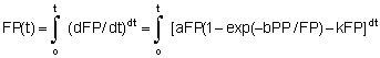
The first term describes the increase in the fish population as a direct proportion of the existing population and is related exponentially with the quantity of food per fish (PP/FP). The second term (k FP) describes the decrease in fish proportionate to the existing population having normal mortality. The symbols a, b, k are constants that must be estimated in each particular case.
Figure 17. Matrices showing simple qualitative (a) and semiquantitative (b) descriptions of input/output relationships of the effects of a dam on fish production
(a)
|
INPUT (PP) |
OUTPUT (FP) |
|
Increase |
Increase |
|
Decrease |
Decrease |
(b)
|
INPUT (PP) |
OUTPUT (FP) |
|
U max |
Large increase |
|
U max U o |
Small increase |
|
U o |
No change |
|
U o U min |
Small decrease |
|
U min |
Loss of species |
This description is the most precise of the three since, for each numerical value of primary production, one can obtain a numerical value for fish production. Naturally, it does not make sense to represent this description in a tabular form as in Figure 17 since there exists an infinite number of pairs of values for inputs and outputs.
A mathematical description can be much more complex, that is, if the numerous factors that influence the growth of each fish population are considered. This, of course, requires much more information on the population structure of the fish and on the primary producers.
These representations are only three examples of the ways that the internal mechanisms that relate input and outputs of a subsystem can be dealt with. If all of the factors could be represented correctly with mathematical equations, one could easily construct a mathematical model of the total system which would permit predictions to be made with a relatively high precision.
![]()
![]()
![]()
![]()