Caribbean Disaster
Mitigation Project
Implemented by the Organization of American States
Unit of Sustainable Development and Environment
for the USAID Office of Foreign Disaster Assistance and the Caribbean Regional Program


Caribbean Disaster
Mitigation Project |
|
Click here to view / print the figures for this document.
Forward
Executive Summary
Acknowledgements
1.0 Introduction
2.0 The Hurricane Hazard
3.0 Approach to Loss Estimation of Infrastructure
4.0 Physical Documentation and Estimation of Replacement Costs for
the Inventory at Risk
5.0 Estimation of Structural and Content Damage to Infrastructure
6.0 Description of Elements at Risk
7.0 Vulnerability Cures for Buildings
8.0 Wind Hazard in Dominica
9.0 Summary of PML for Dominica
10.0 Elements at Risk and Vulnerability Curves
11.0 Wind HAzard in St. Lucia
12.0 Summary of PML for St. Lucia
13.0 Elements at Risk and Vulnerability Curves
14.0 Wind Hazard in St. Kitts and Nevis
Bibliography
Appendices
Appendix 1: General Documentation [Not currently available in electronic format]
1.0 Report of Trips to Countries (HTML 16k)
2.0 Blank Forms for PML Study (MS Excel 27k)
3.0 Instructions for Entering Building Data for PML Study (HTML 9k)
Appendix 2: Supporting Documentation for Dominica
1.0 Physical Description and Replacement Cost Estimation for Infrastructure of Dominica (PDF 52k) *
2.0 Model Parameters for Buildings and Contents in Dominica (PFD 28k)
3.0 Vulnerability Curves for Dominica Buildings (PDF 30k)
4.0 Summary of PML Analysis for Dominica
- Case 1: 50% Upper Prediction Limit (UPL) MLE 50-Year Mean Return Period Event (PDF 71k) *
- Case 2: 90% Upper Prediction Limit (UPL) MLE 50-Year Mean Return Period Event (PDF 70k) *
- Case 3: 50% Upper Prediction Limit (UPL) MLE 100-Year Mean Return Period Event (PDF 70k) *
- Case 4: 90% Upper Prediction Limit (UPL) MLE 100-Year Mean Return Period Event (PDF 70k) *
5.0 Photographs of Typical Infrastructure Elements in Dominica (PDF 2,328k)
Appendix 3: Supporting Documentation for St. Lucia
1.0 Physical Description and Replacement Cost Estimation for Infrastructure of St. Lucia (PDF 70k) [Excel 145k]*
2.0 Model Parameters for Buildings and Contents in St. Lucia (PFD 32k)
3.0 Vulnerability Curves for St. Lucia Buildings (PDF 60k) [Append 2 and 3: Word 170k]
4.0 Summary of PML Analysis for St. Lucia
- Case 1: 50% Upper Prediction Limit (UPL) MLE 50-Year Mean Return Period Event (PDF 102k) [Excel 210k]*
- Case 2: 90% Upper Prediction Limit (UPL) MLE 50-Year Mean Return Period Event (PDF 102k) [Excel 210k]*
- Case 3: 50% Upper Prediction Limit (UPL) MLE 100-Year Mean Return Period Event (PDF 103k) [Excel 210k]*
- Case 4: 90% Upper Prediction Limit (UPL) MLE 100-Year Mean Return Period Event (PDF 7103k) [Excel 210k]*
5.0 Photographs of Typical Infrastructure Elements in St. Lucia (MS Word 2,563k)
Appendix 4: Supporting Documentation for St. Kitts and Nevis
1.0 Physical Description and Replacement Cost Estimation for Infrastructure of St. Kitts and Nevis (81k)
2.0 Model Parameters for Buildings and Contents in St. Kitts and Nevis (91k)
3.0 Vulnerability Curves for St. Kitts and Nevis Buildings (67k)
4.0 Summary of PML Analysis for St. Kitts and Nevis (66k)
- Case 1: 50% Upper Prediction Limit (UPL) MLE 50-Year Mean Return Period Event (144k)
- Case 2: 90% Upper Prediction Limit (UPL) MLE 50-Year Mean Return Period Event (132k)
- Case 3: 50% Upper Prediction Limit (UPL) MLE 100-Year Mean Return Period Event (141k)
- Case 4: 90% Upper Prediction Limit (UPL) MLE 100-Year Mean Return Period Event (131k)
5.0 Photographs of Typical Infrastructure Elements in St. Kitts and Nevis (1,812k)
Low penetration of catastrophe insurance in the Caribbean is recognized as a significant constraint on sustainable development in a region prone to natural disasters. This low penetration is particularly acute in the regional infrastructure stock, which is still overwhelmingly owned by national governments.
In response to a dramatic tightening of the insurance market following hurricanes Andrew and Iniki in the early 1990s, the heads of government of CARICOM established a Working Party on Insurance and Reinsurance to study critical insurance issues against the background of increased frequency of destructive hurricanes in the region. The OAS, as executing agency of the Caribbean Disaster Mitigation Project (CDMP), and the World Bank joined forces in helping the Working Party to prepare a strategy paper outlining options for strengthening the regional insurance industry, reducing the risk exposure and vulnerability to natural perils, and establishing regional mechanisms to increase risk retention in the region and increase the availability of affordable reconstruction financing. The CDMP is funded by the Office of Foreign Disaster Assistance of the U.S. Agency for International Development (OFDA/USAID)
A critical factor in determining the viability of such financial mechanisms is an accurate understanding of the potential loss associated with a major natural-hazard event in the region. To support this effort, the OAS and the World Bank jointly carried out a pilot study to estimate the probable maximum losses in public infrastructure from credible hurricane events in three Eastern Caribbean countries. The study covers what might be called the lifeline infrastructure that supports social welfare and economic activity: electrical power generation, transmission and distribution facilities, airports, seaports, road network, water and sanitation facilities, waste management sites, schools, and hospitals.
The study compiles a comprehensive inventory of all facilities and structures, estimates replacement values, and estimates loss potential associated with hurricane events associated with 50- and 100- year return periods. The resulting information can be used as a basis for defining reconstruction needs and designing financing mechanisms to meet them. The same information can also be used for determining priorities for retrofitting/reconstruction investment projects.
The World Bank will also use the information from this pilot work on public-sector assets, and from ongoing work on residential and commercial PML estimations, as inputs into a financial model to determine how risk-transfer and reinsurance arrangements (including the use of multi-country catastrophe pooled funds backed by contingent capital) could be optimally structured. The objective is to obtain the broadest possible coverage against catastrophic risks, including reduced pricing volatility, particularly given the vulnerabilities, both real and financial, of small disaster-prone economies.
Jan Vermeiren
Unit for Sustainable Development
and Environment
Organization of American States John Pollner
Finance, Private Sector
& Infrastructure Department
World Bank
A probable maximum loss (PML) estimate is the monetary loss, usually expressed as a percentage of the total value, experienced by a structure or collection of structures when subjected to a "maximum credible event". A maximum credible event may be some natural hazard of a certain magnitude or one with a given probability of occurrence in a stated time period.
The objective of the study was to perform a probable maximum loss (PML) on three Caribbean countries subjected to the hurricane peril. Data to be collected by local engineers for use in the probable maximum loss estimation were defined by the lead consultant based in the U.S.
For each of the countries selected for the study, the following approach was utilized to determine the PML for the infrastructure elements at risk:
Step 1: Defined the infrastructure elements to be included in the study. This step was necessary for at least two reasons. First, it defined the boundary of the problem and second, it determined what data were to be collected. The elements to be included in the study were defined under the terms of reference.
Step 2: Documented the exposure and vulnerability of the infrastructure elements at risk. Exposure relates to the extent of the interaction between the hazard and the element at risk. In this study exposure was related to such items as characteristic terrain roughness and topography. Vulnerability is the resistance or strength of the element. The resistance of the infrastructure element depends upon such factors as age, quality of materials, level of design attention, codes used, and the quality of construction. The resistance of the element at risk is a necessary input for the estimation of the probability of failure of the element. Information on the exposure is necessary for the adjustment of the hazard forces at the site of an infrastructure element.
The data collection instrument included a form for collecting the information accompanied by appropriate guidelines. The information to be collected for each structure type was deemed sufficient to estimate potential losses and replacement values for the following types of facilities: power generation systems, airports, seaports, road networks, water and sanitation systems, waste management systems, and schools and hospitals. The lead consultant traveled to each of the islands included in the study and met with a previously selected local engineer. The purpose of this trip was to instruct the local engineer on the nature of the information to be collected and to review a selected number of the facilities covered by the study.
Step 3: Estimated the replacement cost of the elements at risk. The expected loss is the product of the probability of the loss of the infrastructure element and the replacement cost of that element. Such costs were obtained from owners' records, insurance documents, or cost estimates performed by the local engineering consultant.
Step 4: Generated damageability/vulnerability functions for the elements at risk. From the documentation of the vulnerability of the infrastructure elements at risk and existing models for damage evaluation, the probability of failure/loss of an element was estimated as a function of the magnitude of the hazard. The details of the vulnerability model depend upon the characteristics of the element at risk under consideration. For example the approach and calculation details differ significantly for an airport runway and a hospital. However, for all elements at risk, the output of this step is the probability of loss of the element at risk as a function of hazard magnitude.
Step 5: Selected "Maximum Credible Events" for the locations of interest. Maximum credible events may be described in terms of their mean return periods. The mean return period of a hurricane of magnitude "x" may be defined as the average time interval between hurricanes whose intensity exceeds the value "x". To account for the uncertainty in the prediction of the magnitude of a hazard associated with the mean return period, confidence limits, in the study referred to as upper prediction limits, are used to estimate upper bounds for the magnitude. In this study the four following maximum credible events were selected:
Step 6: Adjusted hurricane wind speeds to the location of the structure by accounting for topography and terrain. Wind speed varies with height and terrain roughness. At the ground level the wind intensity is lower and the airflow is turbulent because of the friction generated by the rough surface of the ground. As the height increases, the frictional effect of the ground decreases and the air move only under the influence of pressure gradients. The ground roughness may be categorized into three classes: (1) flat open country, open flat coastal belts and grasslands; (2) Suburban areas, small towns, city outskirts, wooded areas and rolling terrain; and (3) centers of large cities and very rough hilly terrain. Items (1), (2), and (3) in the last sentence correspond roughly to ANSI/ASCE 7-95 Exposure C, Exposure B, and Exposure A, respectively. The terrain conditions were modeled by ANSI/ASCE 7-95 Exposure C. Wind speed-up effects were also meddled in accordance instructions presented in ANSI/ASCE 7-95.
Step 7: Computed the loss at a specific site. With knowledge of the site specific wind speed (Step 6) and the damageability function for the infrastructure element at risk (Step 4) the probability of loss for that element was next determined. The product of the probability of loss and the replacement cost (Step 3) of the element at risk yielded the loss for the element at the site.
Step 8: Summed losses for all infrastructure elements at risk. For a given precinct or parish, the losses were summed according to common categories, e.g., hospitals, police stations, schools, etc… The total losses was also computed for the country.
Step 9: Assigned PMLs for elements, groups of elements, and the total infrastructure. The PML is the percentage of losses to the total value. This number was computed for groups of elements, e.g., police stations and hospitals, as well as for the entire country.
Vulnerability functions were generated for the various infrastructure elements. The damage to the element resulting from the assigned hazard assigned at that location was computed. In the case of buildings, damage to the structure as well as damage to the contents was estimated. In some cases external equipment was attached to a structure. Without additional information on the details of the equipment, the value developed for the damage to the structure was applied to the damage to the external equipment. The cost of damage to structure, contents, or external equipment was computed by multiplying the probability of failure of the element by the replacement cost of the element. The details of the calculation for all elements in the inventory are listed in the appendices for the four credible events. PML summaries, for the 50% Upper Prediction Limit 50-yr mean return period hurricane, of the results for the three countries are provided in Tables 1, 2, and 3.
In Tables 1 - 3, the infrastructure elements considered are listed in the first column. The replacement costs for the structure, contents, and external equipment for each infrastructure element are listed, respectively, in Columns two, three, and four. Note that the values listed are for all structures in that particular category. The total damages (i.e., to structure, contents, and external equipment) computed for each infrastructure element are listed in Columns five, six, and seven. Total replacement costs and damage is provided in the last row of the table. The percent PML for each infrastructure element is provided in Column eight of the tables. Note that the value in Column eight is obtained using the equation:
| %PML = | Column5 + Column6 + Column7 | X 100 |
| Column2 + Column3 + Column4 |
The %PML for the entire infrastructure is the value in the last row of the Column eight. A summary of the PML for all maximum credible events considered for all three countries are provided in Tables 4-6.
Maximum Credible Event |
Wind Speed (mph) |
Estimated Value of Infrastructure Sampled (EC$) |
Estimated Losses (EC$) |
%PML |
|
Mean Return Period (Years) |
Prediction Limit (%) |
||||
50 |
50 |
106 |
855,636,900 |
377,584,875 |
44.13 |
50 |
90 |
119 |
855,636,900 |
547,905,611 |
64.03 |
100 |
50 |
118 |
855,636,900 |
544,776,895 |
63.67 |
100 |
90 |
134 |
855,636,900 |
583,964,263 |
68.25 |
Maximum Credible Event |
Wind Speed (mph) |
Estimated Value of Infrastructure Sampled (EC$) |
Estimated Losses (EC$) |
%PML |
|
Mean Return Period (Years) |
Prediction Limit (%) |
||||
50 |
50 |
100 |
1,198,899,852 |
149,277,163 |
12.45 |
50 |
90 |
116 |
1,198,899,852 |
428,698,392 |
35.76 |
100 |
50 |
113 |
1,198,899,852 |
411,713,725 |
34.34 |
100 |
90 |
136 |
1,198,899,852 |
555,673,928 |
46.35 |
Maximum Credible Event |
Wind Speed (mph) |
Estimated Value of Infrastructure Sampled (EC$) |
Estimated Losses (EC$) |
%PML |
|
Mean Return Period (Years) |
Prediction Limit (%) |
||||
50 |
50 |
102 |
836,471,020 |
200,027,450 |
23.91 |
50 |
90 |
119 |
836,471,020 |
425,210,448 |
50.83 |
100 |
50 |
113 |
836,471,020 |
399,045,303 |
47.71 |
100 |
90 |
133 |
836,471,020 |
471,193,084 |
56.33 |
Firstly, the author wishes to thank the Organization of American States and the World Bank for the opportunity to participate in this important study. Special appreciation is extended to Jan Vermeiren, Principal Specialist of the Unit for Sustainable Development and Environment of the OAS, and John Pollner, Senior Financial Sector Specialist of the Finance, Private Sector & Infrastructure Department of the World Bank for their guidance and advice at critical points in the project. Special appreciation is also extended to Steven Stichter and Charlene Charles of the OAS, for organizing the project and coordinating the efforts of the consulting engineers in the Caribbean. Secondly, the author wishes to acknowledge the crucial contribution of the following consulting engineers: Isaac Baptiste of Dominica, Egbert Louis of St. Lucia, and Lawrie Elmes of St. Kitts and Nevis. Their documentation of the inventory at risk is crucial to the credibility and accuracy of this study. Thirdly, the author thanks Chuck Watson and Ross Wagenseil from Watson Technical Consulting Inc., who produced the comprehensive statistical data on the hurricane hazard for the selected sites under a study commissioned by the OAS. Lastly, appreciation is extended to my immediate colleagues Gladys Higgins, Dr. Sanghyun Choi, Dr. Sooyong Park, and Professor Dale C. Perry without whose contribution to travel arrangements, typesetting, computer programming, reliability analysis, wind engineering, and probabilistic methods, this study would not have converged.
For the purposes of this document, a Probable Maximum Loss is an estimate of the monetary loss, expressed as a percentage of the total value, experienced by a structure or collection of structures when subjected to a "maximum credible event". The maximum credible event is usually some natural hazard of a certain magnitude or one with a given probability of occurrence in a given time period. In this study, the hazard of interest is the hurricane peril thus the maximum credible events will be tied to magnitudes and probabilities of occurrences of wind speeds, wave heights, and surge heights. The maximum credible events used in this study are discussed in the next chapter.
At a minimum, a PML should satisfy the following requirements: (1) reflect local building practices, (2) reflect the existing condition of the structures, (3) reflect the level of professional design attention received by the structures, (4) reflect the local topography and terrain, and (5) reflect the characteristics of the specific materials used in the construction.
The Organization of American States (OAS) developed the terms of reference and contracted a lead international consultant and three engineers each based in one of the selected countries. The abridged terms of reference for the lead consultant were as follows:
"Since its inception, the Caribbean Disaster Mitigation Project (CDMP) has worked with the property insurance industry in the Caribbean to promote loss reduction incentives and hazard mitigation. The large dependency of Caribbean firms on reinsurers outside of the region has hindered progress in this activity. The World Bank and the GS/OAS, through the CDMP, have investigated the possibility of establishing a regional reinsurance fund. Critical to determining the viability of such a fund is an understanding of the potential loss associated with a major natural hazard event in the region. To assist in this effort, estimates of the probable maximum losses in public infrastructure from major hurricane events will be developed under this contract. These estimates will focus on the countries of Dominica, Saint Kitts and Nevis, and Saint Lucia.
Under this contract, the consultant will:
The generic terms of reference for each of the locally-based consultants were as follows:
Under this contract, the (local) consultant will:
The objective of this report is to present the results of the probable maximum loss study for Dominica, St. Lucia, and St. Kitts and Nevis. Potential losses will be reported by infrastructure classification (e.g., schools, ports, etc.) as well as by damage classification (e.g., structural, contents, etc.). Please note that all costs reported in this document are in Eastern Caribbean Dollars.
The remainder of the report is organized into four major sections. Part I includes a description of the hurricane hazard, an explanation of the approach used to estimate the losses to the infrastructure, and a description of how the physical inventory at risk was documented and how the associated replacement cost of the inventory was estimated. Part II includes a description of the PML estimates for Dominica. The section include a description of the elements at risk in Dominica, vulnerability curves for selected elements at risk, a definition of the hazard at specific towns in Dominica, and a summary of the PML calculations for several "maximum credible " events. Part III and Part IV include, respectively, a description of the PML estimates for St. Lucia and St. Kits and Nevis. The references cited in the work are listed in Part V.
The supporting documentation for the study is assembled in Part VI- the appendices. Appendix I contains items such as instructions and data collection forms that are generic to the study. Appendix II contains the information that supports the PML calculation for Dominica. The appendix contains the documentation of the inventory at risk in Dominica, a summary of the data processing of the information, the results of the PML estimates for several maximum credible events, and a set of photographs depicting a sample of the inventory at risk. Appendix III and Appendix IV contain the analogous material for St. Lucia and St. Kitts and Nevis.
The major hazards associated with hurricanes are wind, flying debris, wave action, surge, and rainfall. These hazards can in turn generate other dangerous hazards such as floods, erosion and mudslides. Although the main hazard to be addressed in this study is wind, the impact of surge and wave action will be seriously considered for coastal structures. In addition, once a hurricane of a given magnitude and direction has arrived, the wind speed magnitude may be appropriately modified to reflect such factors as topography, exposure, and potential sheltering from topographic features.
Climatic events such as extreme winds, surge, and wave action are conveniently described using the concept of mean return period. Let x1, x2,�,xn be a set of recorded random extreme values for a period of one year. The measured values may be wind speeds, wave heights, or surge levels. The probability that the random intensity, X, of the wind speed, wave height, or surge level is less than a specific value x, in any one year, is given by
Equation 2.1
P(X < x) = F(x)
Where F(x) is the cumulative distribution function of X. The distribution F(x) is also referred to as the distribution of annual extremes. The return period of a value x, denoted T(x), is defined as the time interval between phenomena whose intensity exceeds x (Ghiocel and Lungu, 1972). Note that the return period T(x) is a random variable. The mean return period, denoted t (x), is the mean value of T(x). It can be shown that the mean return period and the distribution of annual extremes are given by (Ghiocel and Lungu, 1972).
Equation 2.2
t (x) = 1 / (1 - F(x))
Thus the cumulative distribution function of the annual extremes can be related numerically to the magnitude of the mean return period, expressed in years, as
Equation 2.3
F(x) = 1 - 1 / t (x)
The relationship between the cumulative distribution function and the mean return period is demonstrated in Table 2.1. If F(x) is known for wind speeds, surge levels, or wave heights at some location, the hazard may be described probabilistically in terms of the mean return period. Thus from Table 2.1, The probability of a hurricane with a 100 year mean return period will occur in any singly year is 0.01. In other words, the mean return period links the probability of occurrence and the magnitudes of extreme events. Maximum credible events will be identified by their mean return periods.
| t (x) years | 1 | 2 | 5 | 10 | 20 | 25 | 50 | 100 | 200 | 500 | 1000 | 2000 | 10000 |
| F(x) | 0 | 0.5 | 0.8 | 0.9 | 0.95 | 0.96 | 0.98 | 0.99 | 0.995 | 0.998 | 0.999 | 0.9995 | 0.9999 |
Johnson and Watson (1998) have recently completed a comprehensive study of return period estimation of the hurricane peril in the Caribbean. Their results consist of mean return periods for wind, wave, and storm surge for the entire region. Maximum likelihood estimates were computed for a two-parameter Weibul distribution at specified locations using 112 years of meteorological data. In order to account for uncertainties in the meteorological forecast, Johnson and Watson (1998) reported an upper perdition limit with the hazard magnitudes associated with a particular mean return period. A typical set of results for a specific location is presented in Table 2.2. The following direct quote from Johnson and Watson (1998) best explains the concept of the upper prediction limits.
"The MLE (maximum likelihood estimate) column provides the best estimate as to the most likely extreme one minute-ten meter sustained wind for the various time frames. The MLEs are approximately equal to the "median" or 50% values (in knots). This implies that roughly speaking, the MLE is too low about half the time and too high the other half the time. From a planning standpoint, one might wish to "hedge one's bets" to protect against worse than expected phenomena. The 75%, 90%, 95%, and 99% columns are useful for this purpose. For example, 66.0 knots is given for the 95% upper prediction limit for the 10-year return period. Although the best guess of extreme wind in the next ten years is 57 knots, there is only a 1 in 20 chance (corresponding to the 95% level) that the extreme wind will exceed 66 knots. The difference between the 57 and 66 knot wind values reflect the inherent uncertainty in predicting return periods values."
MLE |
50% |
75% |
90% |
95% |
99% |
|
10 year |
57 |
58.2 |
61.2 |
63.9 |
66.0 |
70.4 |
20 year |
76 |
77.0 |
81.6 |
86.7 |
90.6 |
104.4 |
30 year |
89 |
90.5 |
97.0 |
105.0 |
111.4 |
130.4 |
40 year |
102 |
103.1 |
112.8 |
124.0 |
133.1 |
157.8 |
In this study the following four maximum credible events are selected:
Magnitudes of the estimates have been provided by Johnson and Watson (1988) for the following locations:
The data for the specific location will be presented with the analysis of the appropriate country.
For each of the countries selected for the study, the following approach will be utilized to determine the PML for the infrastructure elements at risk
Step 1: Define the infrastructure elements to be included in the study. This step is necessary for at least two reasons. First, it defines the boundaries of the problem and second, it determines what data are to be collected. The elements to be included in the study should be made at the executive level. The outcome of this step should be a detailed listing of the infrastructure elements to be included in the study.
Step 2: Document the exposure and vulnerability of the infrastructure elements at risk. Exposure relates to the extent of the interaction between the hazard and the element at risk. In this study exposure is related to such items as characteristic terrain roughness and topography. Vulnerability is the resistance or strength of the element. The resistance of the infrastructure element depends upon such factors as age, quality of materials, level of design attention, codes used, and the quality of construction. The resistance of the element at risk is necessary for the estimation of the probability of failure of the element. Information on the exposure is necessary for the adjustment of the hazard forces at the site of an infrastructure element.
Step 3: Estimate the replacement cost of the elements at risk. The expected loss is the product of the probability of the loss of the infrastructure element and the replacement cost of that element. Such costs can be obtained from owners' records, insurance documents, or estimates of building professionals.
Step 4: Generate damageability/vulnerability functions for the elements at risk. From the documentation of the vulnerability of the infrastructure elements at risk and existing models for damage evaluation, the probability of failure/loss of an element may be estimated as a function of the magnitude of the hazard. The details of the damageability model will depend upon the characteristics of the element at risk under consideration. For example, the approach and calculation details will differ for an airport runway and a hospital. However, for all elements at risk, the output of this step will be the probability of loss of the element at risk as a function of hazard magnitude.
Step 5: Select a "Maximum Credible Event" for the location of interest. The maximum credible events were discussed in the last chapter. These events describe the intensity of the hurricane without any consideration of modifications to the wind field due to terrain or topography.
Step 6: Adjust hurricane wind speeds to the location of the structure by accounting for topography and terrain. Wind speed varies with height and terrain roughness. At the ground level the wind intensity is lower and the airflow is turbulent because of the friction generated by the rough surface of the ground. As the height increases, the frictional effect of the ground decreases and the air move only under the influence of pressure gradients. The ground roughness may be categorized into three classes: (1) flat open country, open flat coastal belts and grasslands; (2) Suburban areas, small towns, city outskirts, wooded areas and rolling terrain; and (3) centers of large cities and very rough hilly terrain. Items (1), (2), and (3) in the last sentence correspond roughly to ANSI/ASCE 7-95 Exposure C, Exposure B, and Exposure A, respectively.
Step 7: Compute the loss at a specific site. With knowledge of the site specific wind speed (Step 6) and the damageability function for the infrastructure element at risk (Step 4) the probability of loss for that element can now be determined. The product of the probability of loss and the replacement cost (Step 3) of the element at risk yields the loss for the element at the site.
Step 8: Sum losses for all infrastructure elements at risk. For a given precinct or parish, the losses can be summed according to common categories, e.g., hospitals, police stations, schools, etc… The total losses can also be computed for the town, city, or country.
Step 9: Assign PML's for elements, groups of elements, and the total infrastructure. The PML is the percentage of losses relative to the total value of the assets. This number can be computed for groups of elements, e.g., police stations and hospitals, as well as for the entire country.
Approximately ten different forms specially tailored to fit the region were designed and mailed electronically to all local consultants. In the case of buildings, for example, the form requested information such as building location, year built, elevation, code used, number of stories, construction quality, roof details, wall framing, materials, absence or existence of window protection, foundation type, surrounding terrain, and debris hazard. A set of the forms is listed in Appendix I.
A set of instruction for filling out the most complicated form was also provided to the consultants in late August 1998. The entries in the form reflected building material and practices, and codes used in those regions of the Caribbean. A copy of the instruction form is provided in Appendix I.
In accordance with the Terms of Reference, a 2-3 day field trip was made to each designated country. Any outstanding questions were discussed along with any features peculiar to that country. On the first trip Dominica and St. Lucia were visited. St. Kitts was visited on the second trip. Reports summarizing the two trips are provided in Appendix I.
An essentially completed set of data forms was submitted by the consultant from St. Lucia in October, 1998. A completed set of forms was submitted by the consultant from Dominica in November, 1998. An essentially completed set of data forms was submitted by the consultant from St. Kitts in mid April, 1999.
One common way to express the damageability of an infrastructure element is to utilize a so-called loss function (also referred to as a damageability function, vulnerability function, or damage function). In order to relate physical damage to the infrastructure to other socio-economic issues, damage is expressed in terms of economic loss; the greater the damage, the greater the loss. One common measure of damage is the cost to repair the element at risk divided by the replacement cost of the element. This number is referred to as the damage ratio. Once this ratio is calculated, as a function of wind speed, water speed, wave height or surge level, the economic loss can then be estimated, provided the cost to replace the element at risk is known. This line of thinking holds for buildings, roads, transmission lines, or any arbitrary structure.
The model that is used here to estimate damage to a building in a wind environment assumes that a building may be broken down into the following components: roof covering, roof decking, roof framing, roof to wall connection, exterior cladding, openings, lateral bracing, frame-foundation connection, and the foundation itself. The damage to a building is a complex mixture of the damage to the components of the building.
In the model used in this study (Stubbs, 1995), the mean damage ratio drs (i.e., the repair cost divided by the replacement cost of the structure) is given by:
Equation 5.1
where
| v | = | the wind speed at site, |
| = | the triangular density function for the resistance of the ith building component (for the building class) to wind speed, | |
| wi | = | the relative weight of the ith component, |
| as | = | a parameter which defines which type of system defines the behavior of the building, and |
| NC | = | the number of building components in the structural damage ratio model. |
Note that
Equation 5.2

and
Also note that if as as goes to infinity, the building behaves as a series system. That is, failure occurs if any one building component fails. On the other hand, if as as goes to negative infinity, the building behaves as a parallel system and all building components must fail for the building to fail.
The model that is used here to estimate the damage to the contents of the structure is based on the assumption that damage to the contents is caused by damage to the building. Content damage may result from damage to any component of the building discussed in the latter paragraph. The content damage ratio, drc, (i.e., repair cost divided by the replacement cost of the contents) is given by (see, Stubbs and Perry, 1999):
Equation 5.3

where
| pi(v) | = | the structural damage (from Equation 5.1) sustained by the ith component at wind speed v, |
| = | the density function for the resistance of the contents given damage to the ith building component for the building class, | |
| �i | = | a parameter which models the exposure of the contents |
| Ci | = | the relative weight of the ith mode of content damage, |
| ac | = | a parameter which defines the behavior of the content damage modes as a system, and |
| M | = | the number of content damage modes. |
Again, note that
Equation 5.4

and
To aid in the estimating of content damage, ISO has suggested a scheme which classifies
the vulnerability of contents as a function of building usage and material. The scheme is
shown in Table 5.1. Note that a higher risk, in Table 5.1,
implies a higher vulnerability of contents. Four sets of parameters which reflect high,
medium high, medium low, and low risk grades, respectively, are listed in Tables 5.2 to
5.5. Note that the parameters b1 and b2 reflect the level of structural damage at which
damage to the contents begin to occur (b1) and at which the contents are completely
destroyed (b2). Note also that these values vary with the mode of failure. For example, in
the case of high risk grade contents (Table 5.2), damage to
contents may begin as soon as damage to the roof covering commences (e.g., as a result of
water penetration). However, in the case of damage to the roof-wall connection, structural
damage to that element may be substantial (b1 = 0.25) before damage to the contents
ensues. In Table 5.4 and Table
5.5, the reader may note that the parameter b2 is assigned values greater than unity.
Physically, the maximum value of structural damage in a given mode is one. Therefore, if ![]() is the cumulative distribution function of the content damage in mode
i, the maximum content damage is equal to .
is the cumulative distribution function of the content damage in mode
i, the maximum content damage is equal to .
Pavements consist of such items as airport runways, paved and unpaved roads, and concrete pavements (See, e.g., Huang, 1993). A typical paved road may consist of surface asphalt wearing course which overlays another asphalt base course. The asphalt layers are supported by a base (e.g., crushed stone), which may be supported by in situ soil. Modern airport runways are concrete pavements supported by a base or sub base course on local soil.
In a hurricane-prone region, pavements are particularly susceptible to storm-induced erosion processes. At least two prominent failure modes have been identified (Davidson et al 1993): (1) where the layer of (V) and erosion (E).
The various pavement types encountered in this study are listed in Table 5.7. A judgment of the relative resistance of each and every pavement type is listed in the second column. These values are taken to be in the same units as those used in Table 5.6.
A qualitative assignment of the pavement failure probability is given by the twenty five rules summarized in Table 5.8. Note that if the pavement system resistance is equal to the erosion potential, a likelihood of H (High) is assigned. Finally, Table 5.9 provides a quantitative assignment of the qualitative likelihoods. The assignment system essentially assigns a different order of magnitude to each qualitative level. The application of the methodology to the runway systems for the two airports in Dominica is provided in Table 5.10.
If the resistance (strength), R of a utility pole can be expressed by the random variable with density function fR(v), where v is the wind speed, and if the pole is subjected to a deterministic wind speed of magnitude s, then the failure probability of the pole is given
Equation 5.5
Thus if fR(v) is known, pf can be estimated. A rationale for estimating the density function fR(v) is presented below.
Let the design wind speed for the pole be given by vd. Then, if F.S. is the factor of safety used in the design of the pole, wind speed at failure of the pole is given by
Equation 5.6
(Note that the square root results from the relationship between pressure and the square of the wind speed.) Assume that a coefficient of variation v (i.e., standard deviation of design wind speed/ mean of design wind speed), is associated with the design and construction, then a standard deviation associated with the failure speed may be given by
Equation 5.7
Finally, treating vf as a mean, and assuming that the resistance is normally distributed, the failure probability of a pole or transmission tower can be estimated from a knowledge of the design wind speed, assuming values of a factor of safety, and a coefficient of variation for the design and construction. Ellingwood et al (1982) provide guidelines for selecting coefficients of variation for various types of construction.
Wastemanagement collection bins and vehicles are treated as objects that fail by overturning. The overturning moment of the wind force is resisted by the moment of the force equivalent to the weight of the bin or vehicle.
The majority of piers and wharves encountered in this study are pile structures. The only design information provided by the local consultants is the design wave height (Hd) of the structure. In order to estimate the failure probability of a particular pile structure with such limited information, the following approach is utilized.
(1) Estimate the design moment of a pile that can withstand the designated design wave height in a wind environment of 120 mph. That is,
Equation 5.8
Mdesign = M (Hd, vd)
Note that 120 mph is a typical design wind speed specified by codes for the region and for the type of structure.
(2) Estimate the failure resisting moment by assuming a factor of safety. That is,
Equation 5.9
Mfailure = F.S. Mdesign
(3) Assume a coefficient of variation(cov) for the design and construction process.
(4) Estimate a standard deviation of the failure moment, using the equation
Equation 5.10
(5) Treat failure moment as a random variable with mean Mfailure and standard
deviation ![]() .
.
(6) Compute moment induced, Ms, on the pile due to wave action, drag, and impact in a given wind environment (See, e.g. FEMA,
1986).
(7) Estimate the failure probability of the wharves using the equation:
Equation 5.11
Pf = P[Ms > Mfailure]
| Content | Risk Grade |
Risk Grade ID |
| Antiques | High |
1 |
| Aquarium | High |
1 |
| Glassware | High |
1 |
| Open Stock | High |
1 |
| Electronic Equipment | Medium High |
2 |
| Grocery Stores | Medium High |
2 |
| Hospitals | Medium High |
2 |
| Furniture & Fixtures | Medium Low |
3 |
| Department Stores | Medium Low |
3 |
| Hotel | Medium Low |
3 |
| Generators | Low |
4 |
| Grain | Low |
4 |
| Heavy Machinery | Low |
4 |
| Rubber | Low |
4 |
| Vaults | Low |
4 |
| Component | b11 |
b22 |
| Roof Covering | 0 |
0.5 |
| Roof Decking | 0 |
0.5 |
| Roof Framing | 0 |
0.5 |
| Roof-Wall Connection Suct. | 0.25 |
1 |
| Roof-Wall Connection Intp. | 0.25 |
1 |
| Lateral Bracing | 0.25 |
1 |
| Openings | 0 |
0.5 |
| Claddings | 0 |
0.5 |
| Frame-Foundation Connection | 0.25 |
1 |
| Foundation | 0.25 |
1 |
| Gross Structure | 0.25 |
1 |
1Effective level of structural damage at which content damage begins
2Effective level of structural damage at which content damage is 100%
| Component | b1 |
b2 |
| Roof Covering | 0.05 |
1 |
| Roof Decking | 0.05 |
1 |
| Roof Framing | 0.05 |
1 |
| Roof-Wall Connection Suct. | 0.4 |
1 |
| Roof-Wall Connection Intp. | 0.4 |
1 |
| Lateral Bracing | 0.4 |
1 |
| Openings | 0.05 |
1 |
| Claddings | 0.05 |
1 |
| Frame-Foundation Connection | 0.4 |
1 |
| Foundation | 0.4 |
1 |
| Gross Structure | 0.4 |
1 |
| Component | b1 |
b2 |
| Roof Covering | 0.05 |
2 |
| Roof Decking | 0.05 |
2 |
| Roof Framing | 0.05 |
2 |
| Roof-Wall Connection Suct. | 0.5 |
1.45 |
| Roof-Wall Connection Intp. | 0.5 |
1.45 |
| Lateral Bracing | 0.5 |
1.45 |
| Openings | 0.05 |
2 |
| Claddings | 0.05 |
2 |
| Frame-Foundation Connection | 0.5 |
1.45 |
| Foundation | 0.5 |
1.45 |
| Gross Structure | 0.5 |
1.45 |
| Component | b1 |
b2 |
| Roof Covering | 0.05 |
3 |
| Roof Decking | 0.05 |
3 |
| Roof Framing | 0.05 |
3 |
| Roof-Wall Connection Suct. | 0.5 |
2.05 |
| Roof-Wall Connection Intp. | 0.5 |
2.05 |
| Lateral Bracing | 0.5 |
2.05 |
| Openings | 0.05 |
3 |
| Claddings | 0.05 |
3 |
| Frame-Foundation Connection | 0.5 |
2.05 |
| Foundation | 0.5 |
2.05 |
| Gross Structure | 0.5 |
2.05 |
Zone Class |
Processes Occurring in Zone* |
Hurricane Category (Saffir/Simpson) |
||||
(1) |
(2) |
(3) |
(4) |
(5) |
||
1 |
Vd, Wa, S,E |
M |
M |
H |
VH |
VH |
2 |
Vd, Wa, S |
L |
L |
M |
M |
H |
3 |
Vd, S |
VVL |
VLL |
L |
L |
M |
4 |
Vd |
VVL |
VVL |
VVL |
VL |
L |
*Vd = Wind, Wa = Wave action, S = Surge, E = Erosion
H = High, M = Medium, L = Low, VL = Very Low, VVL = Very Very Low
Pavement Systems |
Resistance |
Runways < 10 years |
VH |
Runways > 10 years |
H |
Paved Roads |
M |
Undesigned Concrete Surfaces |
M |
Unpaved Surfaces |
L |
Qualitative Erosion Potential VL |
VLL |
VL |
L |
M |
H |
Qualitative Failure Probability |
Quantitative Failure Probability |
VH |
0.5 |
H |
10-1 |
M |
10-2 |
L |
10-3 |
VL |
10-4 |
VLL |
10-5 |
| 50 yr mean | |||||||
1 |
2 |
3 |
4 |
5 |
6 |
7 |
8 |
Length of Runway |
Replacement Cost/Length |
Total Replacement Cost |
Erosion Potential |
Pavement Resistance |
Qualitative Failure Probability |
Quantitative Failure Probability |
Pavement Damage |
50 Yr. Mean Return Period |
|||||||
4,800(a) |
4,000 |
19,200,000 |
H |
VH |
M |
10-2 |
192,000 |
2,500(b) |
3,500 |
8,750,000 |
H |
H |
H |
10-1 |
875,000 |
50 Yr: 90% Confidence |
|||||||
4,800 |
4,000 |
19,200,000 |
H |
VH |
M |
10-2 |
192,000 |
2,500 |
3,500 |
8,750,000 |
H |
H |
H |
10-1 |
875,000 |
100 Yr. Mean Return Period |
|||||||
4,800 |
4,000 |
19,200,000 |
H |
VH |
M |
10-2 |
192,000 |
2,500 |
3,500 |
8,750,000 |
H |
H |
M |
10-1 |
875,000 |
100 Yr: 90% Confidence |
|||||||
4,800 |
4,000 |
19,200,000 |
VH |
VH |
M |
10-2 |
19,200 |
2,500 |
3,500 |
8,750,000 |
VH |
H |
VH |
-5 |
4,375,000 |
(a) Melville Hall (b) Canefield
The physical documentation for airports, electricity generation plants, waste management system, health service facilities, road networks, utility poles, seaports, wharves, primary schools, public buildings, secondary schools, etc.., are documented in Appendix II. In the words of the local consultant, the values of the replacement costs reported were generated using the following rationale:
"Generally public sector buildings are not insured and the few that are insured, their replacement values are understated, given current construction cost. Therefore, in the case of the public buildings, I have used my knowledge and experience in property valuation and of the local construction industry to arrive at replacement values. With respect to contents, the replacement values were determined based on discussions with officials. In the case of the private sector facilities - Electricity generation and Seaports - values given were provided by the respective company or authority. These facilities are all insured."
Digitized photographs of typical structures in Dominica are also provided in Appendix II.
To account for such differences as age, materials, construction quality, size, level of engineering attention received, etc., the buildings must be classified. Building groups in each infrastructure division are analyzed and assigned to a category. For example, essentially all of the buildings in the Dominica inventory fall into three classes.
The first building class, designated Building Type D-1 (a 1-3 story commercial masonry structure), has the following characteristics: (1) the structure was fully engineered, (2) the structure was built between 1958 and 1995, (3) the structure has a gable roof, and (4) in the opinion of the local engineer the structure was of average construction quality. This type of structure was typical for the airports and the electrical generation facilities.
The second building class, designated Building Type D-2 (a 1-3 story commercial masonry structure), has the following characteristics: (1) the structure was fully engineered, (2) the structure was built in 1980, (3) the structure has a flat roof, and (4) in the opinion of the local engineer the structure was of average construction quality. This type of structure was typical for the schools, government buildings, and hospitals.
The third building class, designated Building Type D-3 (a 1-3 story commercial masonry structure), has the following characteristics: (1) the structure was fully engineered, (2) the structure was built between 1982 and 1994, (3) the structure has a gable roof, and (4) in the opinion of the local engineer the structure was of average construction quality. This type of structure was typical for the government buildings.
Using extensive raw data, expert opinion, and engineering calculation, a systematic
method has been developed to assign model parameters to any building class once the type
of information on the PML form has been provided. Examples of such parameters for the
airport building, electricity generation buildings, and the health facilities are provided
in Tables 7.1-7.3. Each table describes the construction
material used for each of the major building elements. For example for Building Type D-1,
the roof covering is provided by metal sheathing. Parameters a1 and a2
are used to define the density function ![]() (i.e., the resistance of
the component) defined in Equation 5.1. Note that the units of a1 and a2
are in miles per hour. Also as discussed in Section 5.3, the parameters b1 and
b2 are used to define the density function
(i.e., the resistance of
the component) defined in Equation 5.1. Note that the units of a1 and a2
are in miles per hour. Also as discussed in Section 5.3, the parameters b1 and
b2 are used to define the density function ![]() (i.e.,
resistance of the contents) in Equation 5.3. Note that the units of b1 and b2
are non-dimensional. The weighing factors Ii and Ji correspond,
respectively, to wi and ci in Equations 5.1 and 5.3. Note that the
units of wi and ci are non-dimensional.
(i.e.,
resistance of the contents) in Equation 5.3. Note that the units of b1 and b2
are non-dimensional. The weighing factors Ii and Ji correspond,
respectively, to wi and ci in Equations 5.1 and 5.3. Note that the
units of wi and ci are non-dimensional.
On using the parameters in the above tables along with the damageability models described in Chapter 5, damageability curves for each of the building classes can be developed. Representative curves corresponding to the three building classes above are presented in Tables 7.4 - 7.6. A graphic of the damageability showing the content and structural damage ratio as a function of wind speed is also presented.
Building Element |
Description |
Model Parameters |
|||||
a1 |
a2 |
b1 |
b2 |
II |
JI |
||
| Roof Covering | Metal Sheathing | 58 |
185 |
0.00 |
0.50 |
3.00 |
3.00 |
| Roof Decking | Metal Decking | 55 |
176 |
0.00 |
0.50 |
3.00 |
3.00 |
| Roof Framing | Concrete Slab | 104 |
231 |
0.00 |
0.50 |
3.00 |
3.00 |
| Roof-wall Connection | Rigid | 76 |
185 |
0.25 |
1.00 |
3.00 |
3.00 |
| Roof-wall (and Intp.) | Rigid | 69 |
177 |
0.25 |
1.00 |
3.00 |
3.00 |
| Lateral Bracing | Shear Wall | 99 |
220 |
0.25 |
1.00 |
0.10 |
0.00 |
| Openings | Not Protected | 55 |
107 |
0.00 |
0.50 |
3.00 |
3.00 |
| Cladding | RC Block | 100 |
241 |
0.00 |
0.50 |
0.10 |
0.00 |
| FF Connection | Rigid | 132 |
220 |
0.25 |
1.00 |
0.10 |
0.00 |
| Foundation | Slab on Grade | 132 |
275 |
0.25 |
1.00 |
0.10 |
0.00 |
| Gross Structure | N/A | 99 |
275 |
0.25 |
1.00 |
0.00 |
0.40 |
* Main features
** 1-minute sustained
Building Element |
Description |
Model Parameters |
|||||
a1 |
a2 |
b1 |
b2 |
II |
JI |
||
| Roof Covering | Metal Sheathing | 58 |
185 |
0.00 |
0.50 |
3.00 |
3.00 |
| Roof Decking | Wooden Planks | 55 |
176 |
0.00 |
0.50 |
3.00 |
3.00 |
| Roof Framing | RC | 104 |
231 |
0.00 |
0.50 |
3.00 |
3.00 |
| Roof-wall Connection | Rigid | 76 |
185 |
0.25 |
1.00 |
3.00 |
3.00 |
| Roof-wall (and Intp.) | Rigid | 69 |
177 |
0.25 |
1.00 |
3.00 |
3.00 |
| Lateral Bracing | RC | 104 |
241 |
0.25 |
1.00 |
0.10 |
0.00 |
| Openings | Not Protected | 55 |
107 |
0.00 |
0.50 |
3.00 |
3.00 |
| Cladding | RC Block | 90 |
241 |
0.00 |
0.50 |
0.10 |
0.00 |
| FF Connection | Rigid | 132 |
220 |
0.25 |
1.00 |
0.10 |
0.00 |
| Foundation | Slab on Grade | 132 |
275 |
0.25 |
1.00 |
0.10 |
0.00 |
| Gross Structure | N/A | 104 |
275 |
0.25 |
1.00 |
0.00 |
0.40 |
* Main features
** 1-minute sustained
Building Element |
Description |
Model Parameters |
|||||
a1 |
a2 |
b1 |
b2 |
II |
JI |
||
| Roof Covering | Metal Sheathing | 58 |
185 |
0.00 |
0.50 |
3.00 |
3.00 |
| Roof Decking | Wooden Planks | 55 |
176 |
0.00 |
0.50 |
3.00 |
3.00 |
| Roof Framing | Wooden Truss | 99 |
220 |
0.00 |
0.50 |
3.00 |
3.00 |
| Roof-wall Connection | Straps | 76 |
185 |
0.25 |
1.00 |
3.00 |
3.00 |
| Roof-wall (and Intp.) | Straps | 69 |
177 |
0.25 |
1.00 |
3.00 |
3.00 |
| Lateral Bracing | Shear Wall | 99 |
220 |
0.25 |
1.00 |
0.10 |
0.00 |
| Openings | Not Protected | 55 |
107 |
0.00 |
0.50 |
3.00 |
3.00 |
| Cladding | Plain Conc. Block | 100 |
241 |
0.00 |
0.50 |
0.10 |
0.00 |
| FF Connection | Rigid | 132 |
220 |
0.25 |
1.00 |
0.10 |
0.00 |
| Foundation | Slab on Grade | 132 |
275 |
0.25 |
1.00 |
0.10 |
0.00 |
| Gross Structure | N/A | 99 |
275 |
0.25 |
1.00 |
0.00 |
0.40 |
* Main features
** 1-minute sustained
Wind Speed (mph) |
Structural Damage Ratio |
Content Damage Ratio |
50 |
0.000000 |
0.000000 |
60 |
0.003653 |
0.000462 |
70 |
0.035084 |
0.037773 |
80 |
0.102899 |
0.175393 |
90 |
0.193886 |
0.220598 |
100 |
0.280575 |
0.323409 |
110 |
0.364680 |
0.444799 |
120 |
0.465530 |
0.515341 |
130 |
0.577037 |
0.611818 |
140 |
0.680010 |
0.749598 |
150 |
0.768098 |
0.870907 |
160 |
0.841296 |
0.954310 |
170 |
0.899188 |
0.977829 |
180 |
0.936545 |
0.980581 |
190 |
0.959014 |
0.984474 |
200 |
0.975817 |
0.989805 |
210 |
0.988098 |
0.994248 |
220 |
0.995705 |
0.997051 |
230 |
0.998837 |
0.998679 |
240 |
0.999348 |
0.999517 |
250 |
0.999668 |
0.999874 |
260 |
0.999880 |
0.999984 |
270 |
0.999987 |
1.000000 |
280 |
1.000000 |
1.000000 |
290 |
1.000000 |
1.000000 |
300 |
1.000000 |
1.000000 |
Wind Speed (mph) |
Structural Damage Ratio |
Content Damage Ratio |
50 |
0.000000 |
0.000000 |
60 |
0.003653 |
0.000462 |
70 |
0.035084 |
0.037773 |
80 |
0.102899 |
0.175393 |
90 |
0.193886 |
0.220598 |
100 |
0.280622 |
0.323409 |
110 |
0.364747 |
0.444799 |
120 |
0.465561 |
0.515341 |
130 |
0.576986 |
0.611818 |
140 |
0.679829 |
0.749598 |
150 |
0.767742 |
0.870907 |
160 |
0.840718 |
0.954310 |
170 |
0.898484 |
0.977566 |
180 |
0.935838 |
0.979877 |
190 |
0.958358 |
0.983320 |
200 |
0.975258 |
0.988574 |
210 |
0.987683 |
0.993545 |
220 |
0.995480 |
0.996691 |
230 |
0.998776 |
0.998517 |
240 |
0.999348 |
0.999457 |
250 |
0.999668 |
0.999859 |
260 |
0.999880 |
0.999982 |
270 |
0.999987 |
1.000000 |
280 |
1.000000 |
1.000000 |
290 |
1.000000 |
1.000000 |
300 |
1.000000 |
1.000000 |

Wind Speed (mph) |
Structural Damage Ratio |
Content Damage Ratio |
50 |
0.000000 |
0.000000 |
60 |
0.003653 |
0.000462 |
70 |
0.035084 |
0.037773 |
80 |
0.102899 |
0.175393 |
90 |
0.193886 |
0.220598 |
100 |
0.280597 |
0.323409 |
110 |
0.366647 |
0.445129 |
120 |
0.470176 |
0.518760 |
130 |
0.584774 |
0.625132 |
140 |
0.691247 |
0.784690 |
150 |
0.783248 |
0.917243 |
160 |
0.860758 |
0.970420 |
170 |
0.918737 |
0.977829 |
180 |
0.953495 |
0.980581 |
190 |
0.972955 |
0.984474 |
200 |
0.986337 |
0.989805 |
210 |
0.994787 |
0.994248 |
220 |
0.998151 |
0.997051 |
230 |
0.998857 |
0.998679 |
240 |
0.999348 |
0.999517 |
250 |
0.999668 |
0.999874 |
260 |
0.999880 |
0.999984 |
270 |
0.999987 |
1.000000 |
280 |
1.000000 |
1.000000 |
290 |
1.000000 |
1.000000 |
300 |
1.000000 |
1.000000 |

The wind data for Roseau, Dominica, utilized in this study is provided in Table 8.1
| Mean Return Period � | Upper Prediction limits |
||||
50% |
75% |
90% |
95% |
99% |
|
| 10 Year | 62.8* |
65.6 |
68.3 |
69.5 |
72.7 |
| 25 Year | 80.1 |
84.0 |
88.3 |
91.7 |
102.2 |
| 50 Year | 92.2 |
97.0 |
103.5 |
109.3 |
125.8 |
| 100 Year | 102.9 |
109.6 |
116.9 |
124.9 |
141.4 |
*1-minute sustained at 10 meters
The credible events selected for this study are
The exposure assumed for the island was Exposure C (see e.g., ANSI/ASCE 7-1995). Exposure C includes open terrain with scattered obstructions having heights generally less than 30ft (9.1m). In addition, the basic wind speed was modified according to building height and topographic effects in accordance with guidelines presented in ANSI/ASCE 7-95. Note that the topographic effects accounted for the wind speed-up effects expected in the island. Values for the topographic effect and the exposure developed in accordance with ANSI/ASCE 7-95 are provided in Appendix II.
Vulnerability functions were generated for the various infrastructure elements, as described in Chapter 5. The damage to the element resulting from the assigned hazard assigned at that location was computed. In the case of buildings, damage to the structure and damage to the contents were estimated. In some cases external equipment was attached to a structure. Without additional information on the details of the equipment, the value developed for the damage to the structure was applied to the damage to the external equipment. The cost of damage to structure, contents, or external equipment was computed by multiplying the probability of failure of the element by the replacement cost of the element. The details of the calculation for all elements in the inventory are listed in Appendix II for the four credible events. Summaries of the results for Dominica are provided in Tables 9.1-9.4.
In Tables 9.1 - 9.4, the infrastructure elements considered are listed in the first column. The replacement costs for the structure, contents, and external equipment for each infrastructure element are listed, respectively, in Columns two, three, and four. Note that the values listed are for all structures in that particular category. The total damages (i.e., to structure, contents, and external equipment) computed for each infrastructure element are listed in Columns five, six, and seven. Total replacement costs and damage are provided in the last row of the table. The percent PML for each infrastructure element is provided in Column eight of the tables. Note that the value in Column eight is obtained using the equation:
| %PML = | Column5 + Column6 + Column7 | X 100 |
| Column2 + Column3 + Column4 |
The %PML for the entire infrastructure is the value in the last row of the Column eight. A summary of the PML for the entire country and for the four "maximum credible" events is provided in Table 9.5
Maximum Credible Event |
Wind Speed (mph) |
Estimated Value of Infrastructure Sampled (EC$) |
Estimated Losses (EC$) |
%PML |
|
Mean Return Period (Years) |
Prediction Limit (%) |
||||
50 |
50 |
106 |
855,636,900 |
377,584,875 |
44.13 |
50 |
90 |
119 |
855,636,900 |
547,905,611 |
64.03 |
100 |
50 |
118 |
855,636,900 |
544,776,895 |
63.67 |
100 |
90 |
134 |
855,636,900 |
583,964,263 |
68.25 |
The physical documentation for airports, electricity generation plants, waste management system, health service facilities, road networks, utility poles, seaports, wharves, primary schools, public buildings, secondary schools, etc., for St. Lucia are documented in Appendix III. Assignment of replacement costs followed procedures similar to those described for Dominica. A set of digitized photographs summarizing the inventory is also included in Appendix III. The classification of building, the assignment of model parameters for the infrastructure elements, and the generation of the vulnerability functions, all follow the procedures outlined for Dominica.
The Wind data for Castries, St. Lucia, utilized in this study is provided in Table 11.1.
| Mean Return Period � | Upper Prediction limits |
||||
50% |
75% |
90% |
95% |
99% |
|
| 10 Year | 59.0* |
62.1 |
64.6 |
66.0 |
71.0 |
| 25 Year | 75.5 |
79.7 |
83.4 |
87.4 |
99.6 |
| 50 Year | 86.8 |
92.7 |
101.0 |
107.7 |
131.1 |
| 100 Year | 98.0 |
105.3 |
117.1 |
126.5 |
162.4 |
*1-minute sustained at 10 meters
The maximum credible events selected for this study are
The exposure assumed for the island was Exposure C (see e.g., ANSI/ASCE 7-1995). Exposure C includes open terrain with scattered obstructions having heights generally less than 30ft (9.1m). In addition, the basic wind speed was modified according to building height and topographic effects in accordance with guidelines presented in ANSI/ASCE 7-95. Note that the topographic effects accounted for the wind speed-up effects expected in the island. Values for the topographic effect and the exposure developed in accordance with ANSI/ASCE 7-95 are provided in Appendix III.
Vulnerability functions were generated for the various infrastructure elements, as described in Chapter 7. The damage to the element resulting from the assigned hazard assigned at that location was computed. In the case of buildings, damage to the structure and damage to the contents were estimated. In some cases, external equipment was attached to a structure. Without additional information on the details of the equipment, the value developed for the damage to the structure was applied to the damage to the external equipment. The cost of damage to structure, contents, or external equipment was computed by multiplying the probability of failure of the element by the replacement cost of the element. The details of the calculation for all elements in the inventory are listed in Appendix III for the four credible events. Summaries of the results for St. Lucia are provided in Table 12.1 to Table 12.5.
Maximum Credible Event |
Wind Speed (mph) |
Estimated Value of Infrastructure Sampled (EC$) |
Estimated Losses (EC$) |
%PML |
|
Mean Return Period (Years) |
Prediction Limit (%) |
||||
50 |
50 |
100 |
1,198,899,852 |
149,277,163 |
12.45 |
50 |
90 |
116 |
1,198,899,852 |
428,698,392 |
35.76 |
100 |
50 |
113 |
1,198,899,852 |
411,713,725 |
34.34 |
100 |
90 |
136 |
1,198,899,852 |
555,673,928 |
46.35 |
The physical documentation for airports, electricity generation plants, waste management system, health service facilities, road networks, utility poles, seaports, wharves, primary schools, public buildings, secondary schools, etc., for St. Kitts and Nevis are documented in Appendix IV. Assignment of replacement costs followed procedures similar to those described for Dominica. A set of digitized photographs summarizing the inventory is also included in Appendix IV. The classification of building, the assignment of model parameters for the infrastructure elements, and the generation of the vulnerability functions, all follow the procedures outlined for Dominica.
The Wind data for Castries, St. Lucia, utilized in this study is provided in Table 14.1.
| Mean Return Period � | Upper Prediction limits |
||||
50% |
75% |
90% |
95% |
99% |
|
| 10 Year | 61.4* |
64.2 |
66.7 |
68.3 |
73.7 |
| 25 Year | 77.2 |
81.4 |
86.4 |
90.7 |
112.4 |
| 50 Year | 88.6 |
94.3 |
103.5 |
111.3 |
140.1 |
| 100 Year | 98.5 |
106.3 |
116.4 |
125.9 |
163.9 |
*1-minute sustained at 10 meters
The credible events selected for this study are
The exposure assumed for the island was Exposure C (see e.g., ANSI/ASCE 7-1995). Exposure C includes open terrain with scattered obstructions having heights generally less than 30ft (9.1m). In addition, the basic wind speed was modified according to building height and topographic effects in accordance with guidelines presented in ANSI/ASCE 7-95. Note that the topographic effects accounted for the wind speed-up effects expected in the island. Values for the topographic effect and the exposure are provided in Appendix IV.
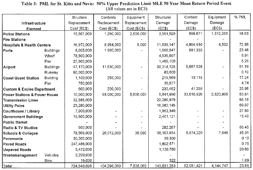
Vulnerability functions were generated for the various infrastructure elements, as described in Chapter 7. The damage to the element resulting from the assigned hazard assigned at that location was computed. In the case of buildings, damage to the structure and damage to the contents were estimated. In some cases external equipment was attached to a structure. Without additional information on the details of the equipment, the value developed for the damage to the structure was applied to the damage to the external equipment. The cost of damage to structure, contents, or external equipment was computed by multiplying the probability of failure of the element by the replacement cost of the element. The details of the calculation for all elements in the inventory are listed in Appendix IV for the four credible events. Summaries of the results for St. Kitts are provided in Tables 15.1-15.5.
Maximum Credible Event |
Wind Speed (mph) |
Estimated Value of Infrastructure Sampled (EC$) |
Estimated Losses (EC$) |
%PML |
|
Mean Return Period (Years) |
Prediction Limit (%) |
||||
50 |
50 |
102 |
836,471,020 |
200,027,450 |
23.91 |
50 |
90 |
119 |
836,471,020 |
425,210,448 |
50.83 |
100 |
50 |
113 |
836,471,020 |
399,045,303 |
47.71 |
100 |
90 |
133 |
836,471,020 |
471,193,084 |
56.33 |
ANSI/ASCE 7-95 (1996), Minimum Design Loads for Buildings and Other Structures, ASCE, New York.
Coastal Construction Manual (1986), FEMA-55 Federal Emergency Management Agency.
Davison, A.T., Borman, C.E., and Nishihara, M., (1994), Hurricanes of 1992: Lessons Learned and Implications for the Future: Proceedings of a Symposium Organized by the American Society of Civil Engineers, December 1-3, 1993, Hyatt Regency Miami City Center at Riverwalk/Edited by Ronald A. Cook and Mehrdad Soltani.
Ellingwood, B., Galambos, T.V., MacGregor, J.G., and Cornell, C.A. (1980), Development of a Probability Based Load Criterion for American National Standard A58, U.S. Department of Commerce.
Ghiocel D., and Lungu, D., (1975), Wind, Snow and Temperature Effects on Structures Based on Probability, Abacus Press, Kent, U.K.
Huang, Y.H., (1993), Pavement Analysis and Design, Prentice Hall, New Jersey.
Johnson, M.E., and Watson, C.C. Jr. (1998), Hurricane Return Period Estimation, 6th Joint Conference on Global Change.
Johnson, M.E., and Watson, C.C. Jr. (1998), Return Period Estimation of Hurricane Perils in the Caribbean, Final Report Submitted to the Organization of American States.
Kandel, A., (1992), Fuzzy Expert Systems, CRC Press, London, U.K.
Stubbs, N. (1995), A White Paper on Hurricane Loss Calculation for the Caribbean Region, Report prepared for the Organization of American States Caribbean Disaster Mitigation Project, Organization of American States, Washington, DC.
Stubbs, N., and Perry, D.C., (1999), Documentation of a Methodology to Compute Structural Damage and Content Damage in a Wind Environment, Final Report Submitted to Department of Civil Engineering, Clemson University, Clemson, SC, Texas Engineering Experiment Station, Contract Number 32525-48800.
| CDMP home page: http://www.oas.org/en/cdmp/ | Project Contacts | Page Last Updated: 19 November 2002 |